BIND-USBL: Bounding IMU Navigation Drift using USBL in Heterogeneous ASV–AUV Teams
Supplementary Material — OCEANS 2026, Sanya
Pranav Kedia¹·², Rajini Makam³, Heiko Hamann¹·², Suresh Sundaram³
¹ Dept. of Computer and Information Science, University of Konstanz, Germany ² Centre for the Advanced Study of Collective Behaviour, University of Konstanz, Germany ³ Dept. of Aerospace Engineering, Indian Institute of Science, Bangalore, India
Take-home message
AUV navigation error is governed mainly by USBL fix availability, not just by USBL fix accuracy. ASV placement and acoustic scheduling must therefore be designed together to keep IMU drift bounded.
- Fix availability matters more than nominal fix accuracy.
- At survey side length L = 140 m, AUV0 coverage improves from 9 % → 79 % when going from 1 ASV to 3 ASVs.
- Mean cross-track error drops from 10.02 m → 0.56 m with 3 ASVs at the same scale.
- End-to-end HF-ping-to-fix-delivery latency stays below 0.57 s across all tested configurations.
Abstract
Accurate and continuous localization of Autonomous Underwater Vehicles (AUVs) in GPS-denied environments is a persistent challenge in marine robotics. In the absence of external position fixes, AUVs rely on inertial dead-reckoning, which accumulates unbounded drift due to sensor bias and noise. This paper presents BIND-USBL, a cooperative localization framework in which a fleet of Autonomous Surface Vessels (ASVs) equipped with Ultra-Short Baseline (USBL) acoustic positioning systems provides intermittent fixes to bound AUV dead-reckoning error.
The key insight is that long-duration navigation failure is driven not by the accuracy of individual USBL measurements, but by the temporal sparsity and geometric availability of those fixes. BIND-USBL combines (i) a multi-ASV formation model linking survey scale and anchor placement to acoustic coverage, (ii) a conflict-graph-based TDMA uplink scheduler for shared-channel servicing, and (iii) delayed fusion of received USBL updates with drift-prone dead reckoning. The framework is evaluated in the HoloOcean simulator using heterogeneous ASV–AUV teams executing lawnmower coverage missions. The results show that localization performance is shaped by the joint interaction of survey scale, acoustic coverage, team composition, and ASV-formation geometry.
Method overview
- ASV formation geometry. ASVs are placed at the vertices of a regular N-gon centred at the survey origin. A closed-form minimum-radius constraint links the survey scale L to the HF acoustic range RHF, giving explicit acoustic-coverage guarantees via a corner-to-nearest-ASV bound.
- Conflict graph and TDMA scheduling. Two AUVs are in acoustic conflict whenever at least one ASV can hear both. A greedy graph colouring of the resulting conflict graph partitions AUVs into ping groups, enabling spatial reuse of the shared HF uplink channel without inter-AUV collision.
- USBL ranging. Each ASV estimates slant range from round-trip travel time and direction of arrival from TDOA across a five-element hydrophone array, fusing with its own GNSS position to produce an absolute AUV fix. When multiple ASVs hear the same AUV, fixes are combined via a minimum-variance linear unbiased estimator, reducing fused-fix standard deviation by 1/√K.
- Complementary filter fusion. Absolute USBL fixes (delayed by acoustic propagation) are fused with relative IMU propagation through a two-step predict–correct scheme. Fixes are stored in a per-AUV min-heap keyed on delivery tick to ensure causal application under variable acoustic delay.
Results
1. Baseline: single-ASV coverage mission at L = 60 m
Multi-AUV boustrophedon coverage at L = 60 m. The single ASV (star) is station-kept at the survey centroid; all four lawnmower strips fall within its HF uplink range.
At this scale, the entire survey area lies within the HF footprint of a single ASV. The TDMA scheduler delivers an aggregate applied fix rate of 0.994 Hz (≈ 298 fixes over 300 s) with near-uniform allocation across AUV0–AUV3 (24.3 %, 25.9 %, 24.4 %, 25.4 %) and end-to-end latency of 51 ms (p95 = 67 ms). This baseline confirms that the protocol services the fleet at the maximum achievable rate on a single shared channel, and that the complementary filter keeps cross-track error sub-metre when coverage is complete.
2. Coverage failure at L = 140 m, single ASV
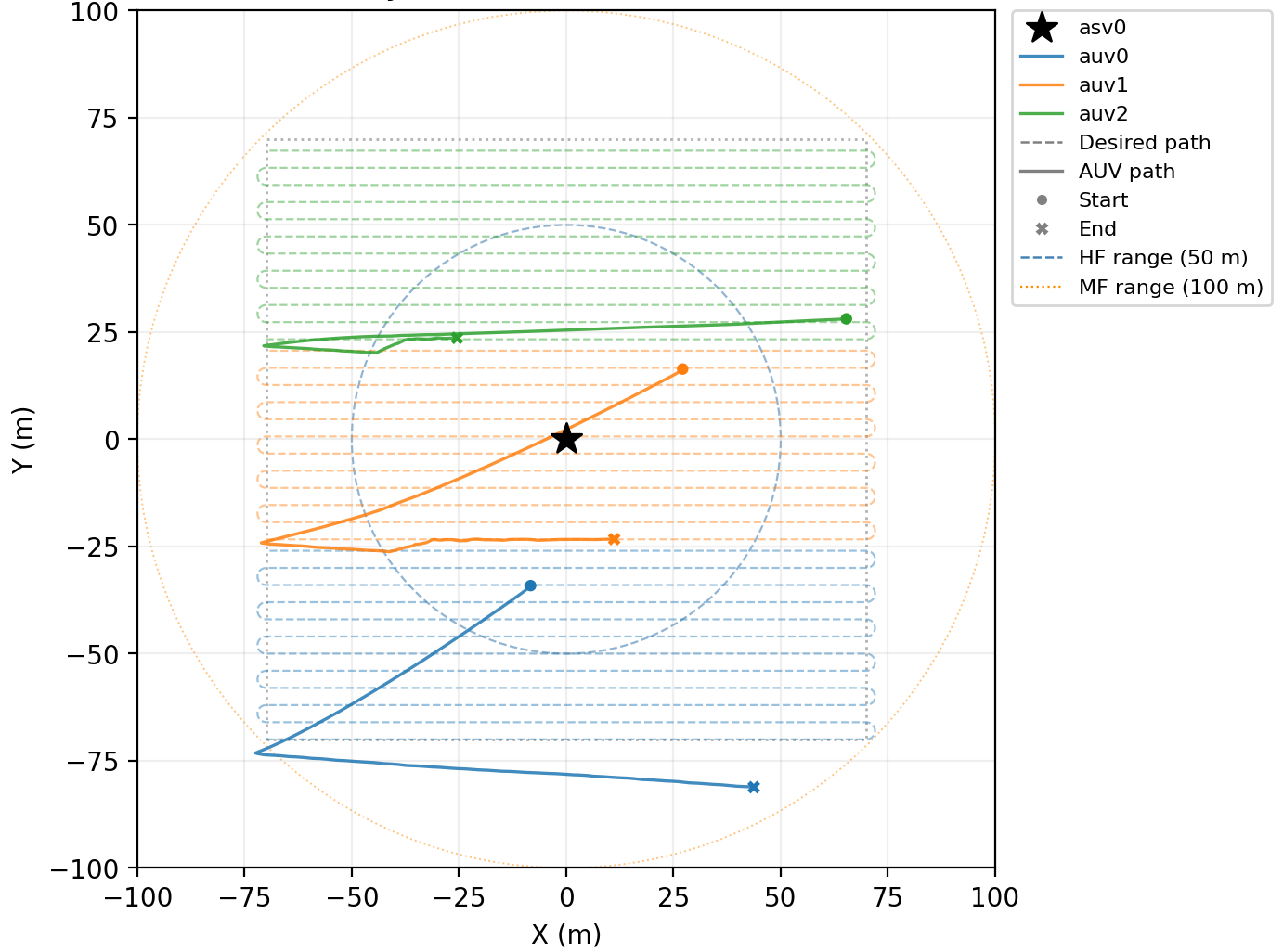
Trajectory overview: L = 140 m, 3 AUVs, 1 ASV (star, α₀ = 0°). The dashed blue circle marks the HF uplink range, the dotted orange circle marks the MF downlink range. The upper lawnmower strip lies almost entirely outside the HF footprint.
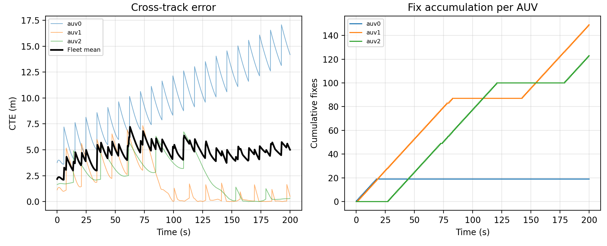
Fleet metrics for the single-ASV failure case. Left: cross-track error over time — AUV0 diverges unboundedly while AUV1–AUV2 stay bounded. Right: cumulative fix count — AUV0’s count flatlines after the first few seconds, characteristic of coverage-limited starvation.
AUV0’s lawnmower strip exits the HF footprint almost immediately and never re-enters it for meaningful durations. It accumulates only 19 fixes over 300 s (9 % coverage) and drifts to a mean CTE of 10.02 m, while AUV1 and AUV2 — operating closer to the centroid — remain bounded.
| Config | AUV | Fixes | Coverage | CTE (m) |
|---|---|---|---|---|
| 1 ASV, 0° | AUV0 | 19 | 9 % | 10.02 |
| 1 ASV, 0° | AUV1 | 149 | 70 % | 1.79 |
| 1 ASV, 0° | AUV2 | 123 | 58 % | 2.52 |
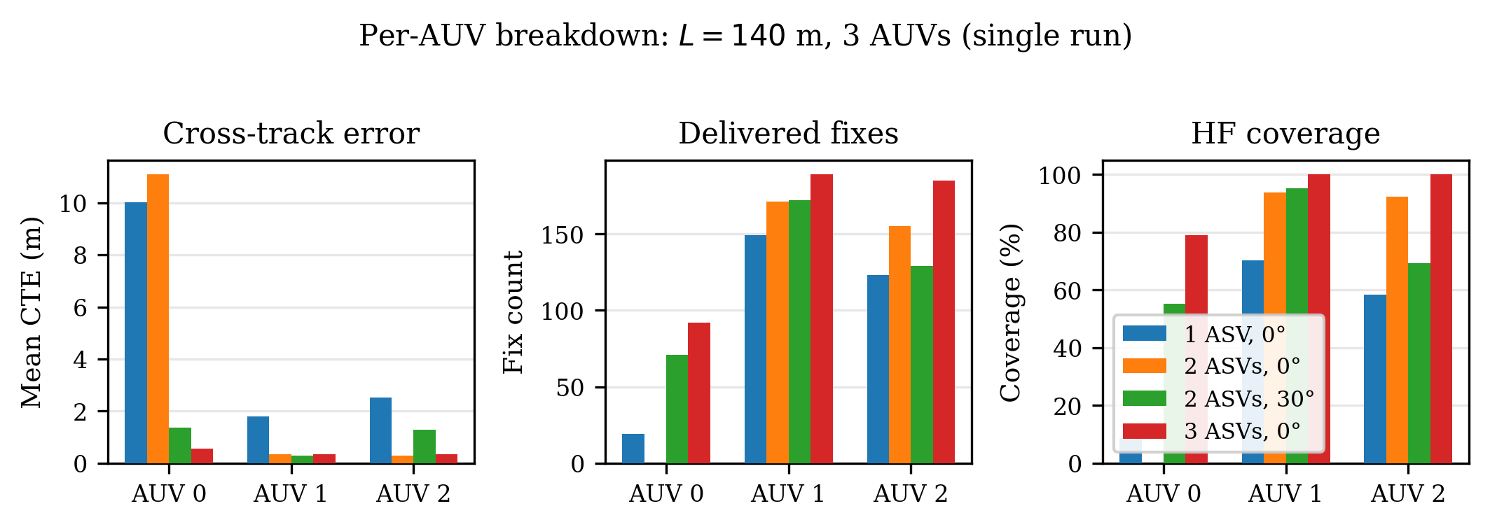
| 3 ASVs, 0° | AUV0 | 92 | 79 % | 0.56 |
| 3 ASVs, 0° | AUV1 | 189 | 100 % | 0.35 |
| 3 ASVs, 0° | AUV2 | 185 | 100 % | 0.35 |
Deploying three ASVs in an equilateral triangle at Rf = RHF recovers AUV0 to 79 % coverage, 92 fixes, and 0.56 m CTE — purely from formation geometry, with no change in hardware or scheduling.
3. Formation angle matters for 2-ASV deployments
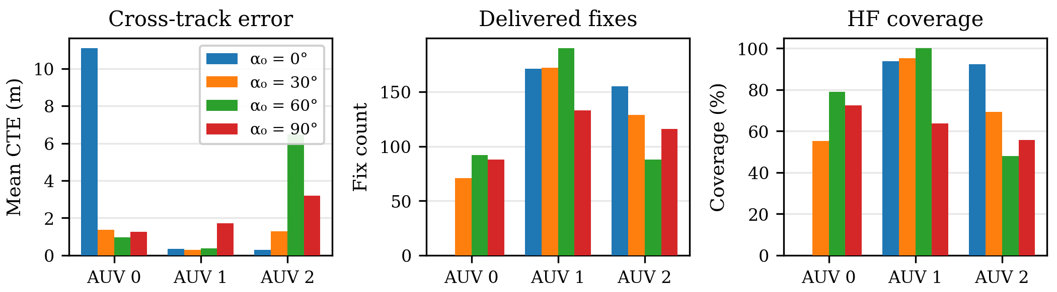
Per-AUV CTE, fix count, and HF coverage for L = 140 m, 3 AUVs, 2 ASVs across formation angles α₀ ∈ {0°, 30°, 60°, 90°}.
At α₀ = 0° the two ASVs align along the x-axis and replicate the same coverage shadow at the y-extremes — AUV0 receives zero fixes and drifts to 11.1 m CTE. A 30° rotation of the formation alone yields an 8× CTE reduction for AUV0, with no change in hardware. For 2-ASV deployments, α₀ is a first-order design variable that can determine mission success or failure.
4. Configuration sweep — design rules
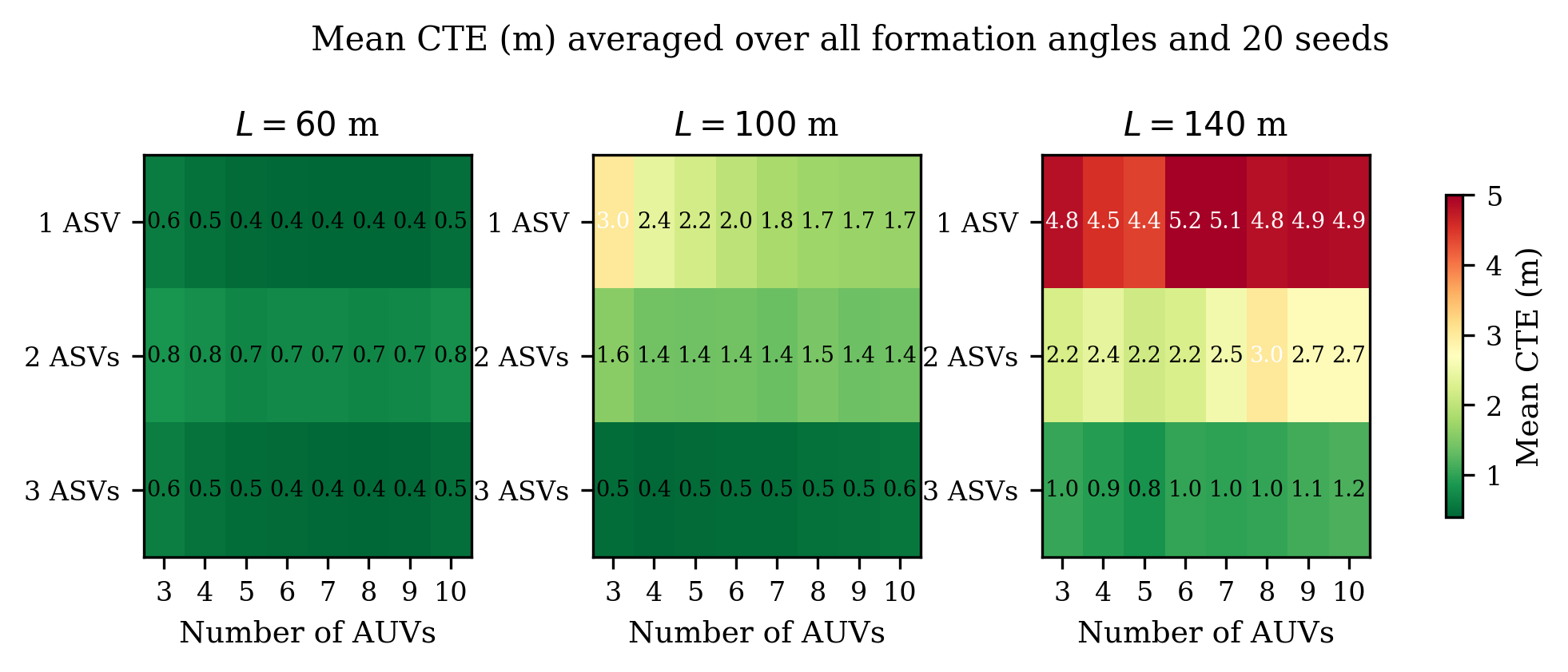
Mean CTE (m) across all formation angles and 20 seeds. Columns: survey side lengths 60, 100, 140 m. Rows: ASV count. Horizontal axis within each cell: AUV count. Green ≤ 1 m (well-localized); red > 4 m (navigation failure).
| L = 60 m | L = 100 m | L = 140 m | |
|---|---|---|---|
| 1 ASV | ✅ Good | ⚠️ Fair | ❌ Poor |
| 2 ASVs | ✅ Good | ✅ Good | ⚠️ Fair |
| 3 ASVs | ✅ Good | ✅ Good | ✅ Good |
Good = coverage ≥ 70 % and mean CTE < 1 m. Fair = 30 % ≤ coverage < 70 % or 1 m ≤ mean CTE < 4 m. Poor = coverage < 30 % or mean CTE > 4 m.
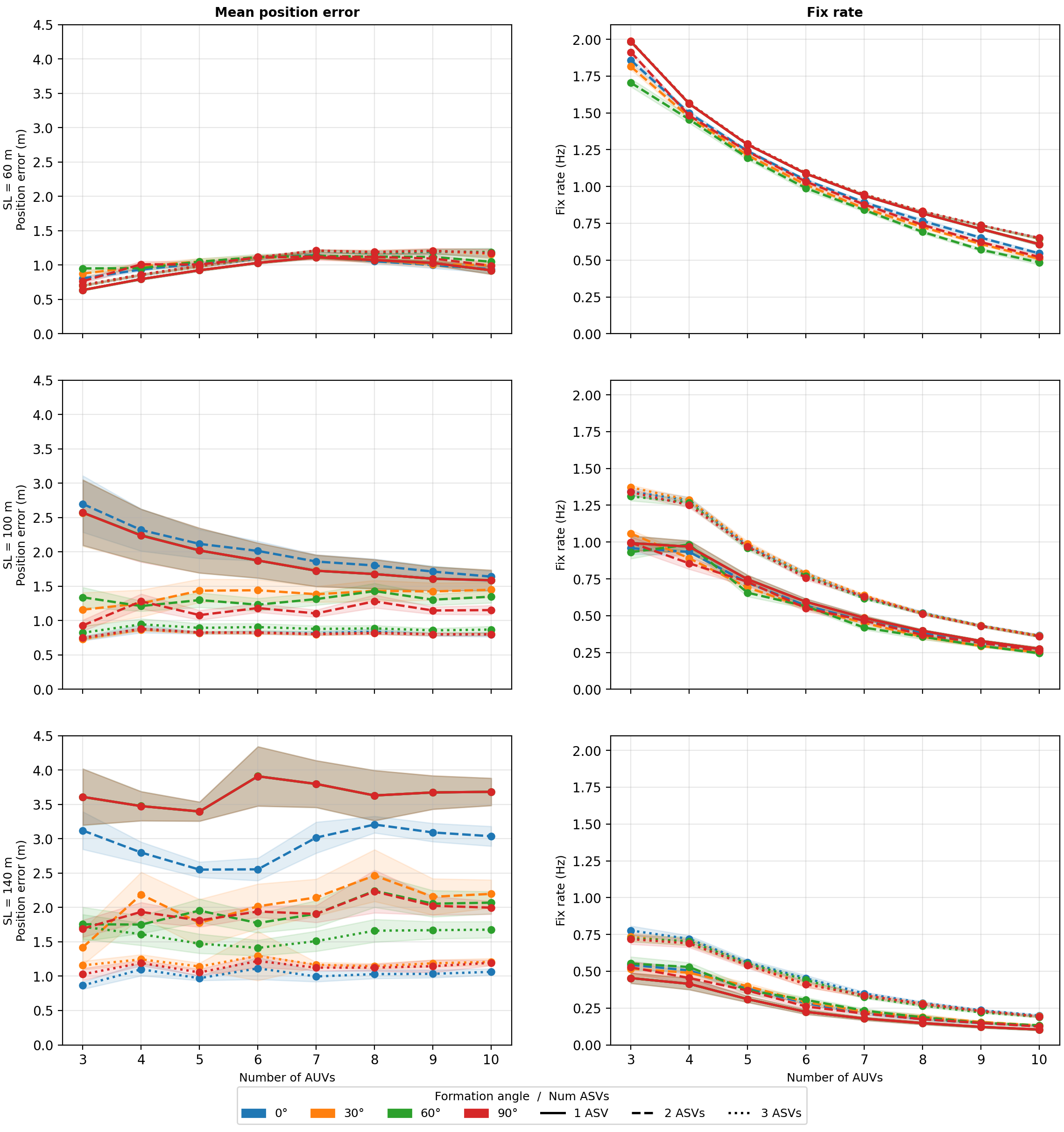
Distance-normalised configuration sweep (20 seeds, mean ±1σ). Left column: mean position error. Right column: applied fix rate. Rows: L = 60, 100, 140 m. Colors denote formation angle; line styles: solid = 1 ASV, dashed = 2 ASVs, dotted = 3 ASVs. The sharp transition from solid to dotted lines at L = 140 m illustrates the binary nature of the coverage threshold.
Three design principles emerge from the sweep:
- Survey scale is the dominant performance factor. Once the survey diagonal exceeds RHF, a single centroid ASV cannot provide full coverage; additional surface anchors are architecturally necessary, not merely beneficial.
- The 1-to-3 ASV transition concentrates the benefit. Going from 1 → 3 ASVs at L = 140 m reduces mean CTE from ~4.8 m to ~1.0 m — a 4–5× reduction.
- Coverage fraction — not fix rate — governs navigation quality. TDMA scheduling reduces per-AUV fix rate monotonically with fleet size, but this does not translate uniformly to CTE growth: it is the binary loss of coverage at survey extremes that dominates.
Downloads
- 📄 Full paper (PDF)
- 🖼️ Graphical abstract / conference poster (PDF) — coming soon
- 💻 Source code & HoloOcean experiments — coming soon
Acknowledgments
PK and HH acknowledge support from DFG through Germany’s Excellence Strategy — EXC 2117 — 422037984 and the Centre for the Advanced Study of Collective Behaviour (CASCB), University of Konstanz. PK and RM acknowledge the use of ChatGPT and Claude for refining academic language and grammar; neither tool was used to generate scientific content.